How to Make a Drop-Down List in Excel: A Comprehensive Guide

Drop-down lists are a powerful excel feature. It’s allowing people to pick an item from a list that you create. Many ways to use it within a spreadsheet. There are some amazing techniques.

Here I cover all these techniques from the most fundamental to the most advanced with easy-to-follow examples.

In this guide, I’m going to start with the fundamentals of how to create a basic drop-down list in Excel for data input.

Basic fundamental for Making a drop-down list in Excel

We use drop-down lists for simple data input. For our example, we already have the Project Names and Start Dates entered.

Now we want to assign a Department to each project and set a project status.

We could manually type in the department name and project status. But using a drop-down list instead makes these inputs way easier. Makes it a way more pleasant user experience and most important. It will ensure data consistency.

To insert a basic drop-down list into a cell, follow these steps:

1. Select the cell where you want to make the drop-down list and go to the Data tab.
2. Click on the Data validation button in the Data Tools section. A small window (Data Validation) opens.
3. In the Data Validation dialogue box, select the List option in the Allow box. Now there’s a new input field that says Source. 
4. In the Source field, you will define the items that will be in your drop-down list. (eg: Production, R&D, Purchase, IT, HR). The simplest approach is to directly enter the items into this field separated by a comma.
5. Once you’re happy with your list, just click Ok.

Now you see this drop-down arrow that allows you to open the drop-down list and select an item that will be inserted into the cell.

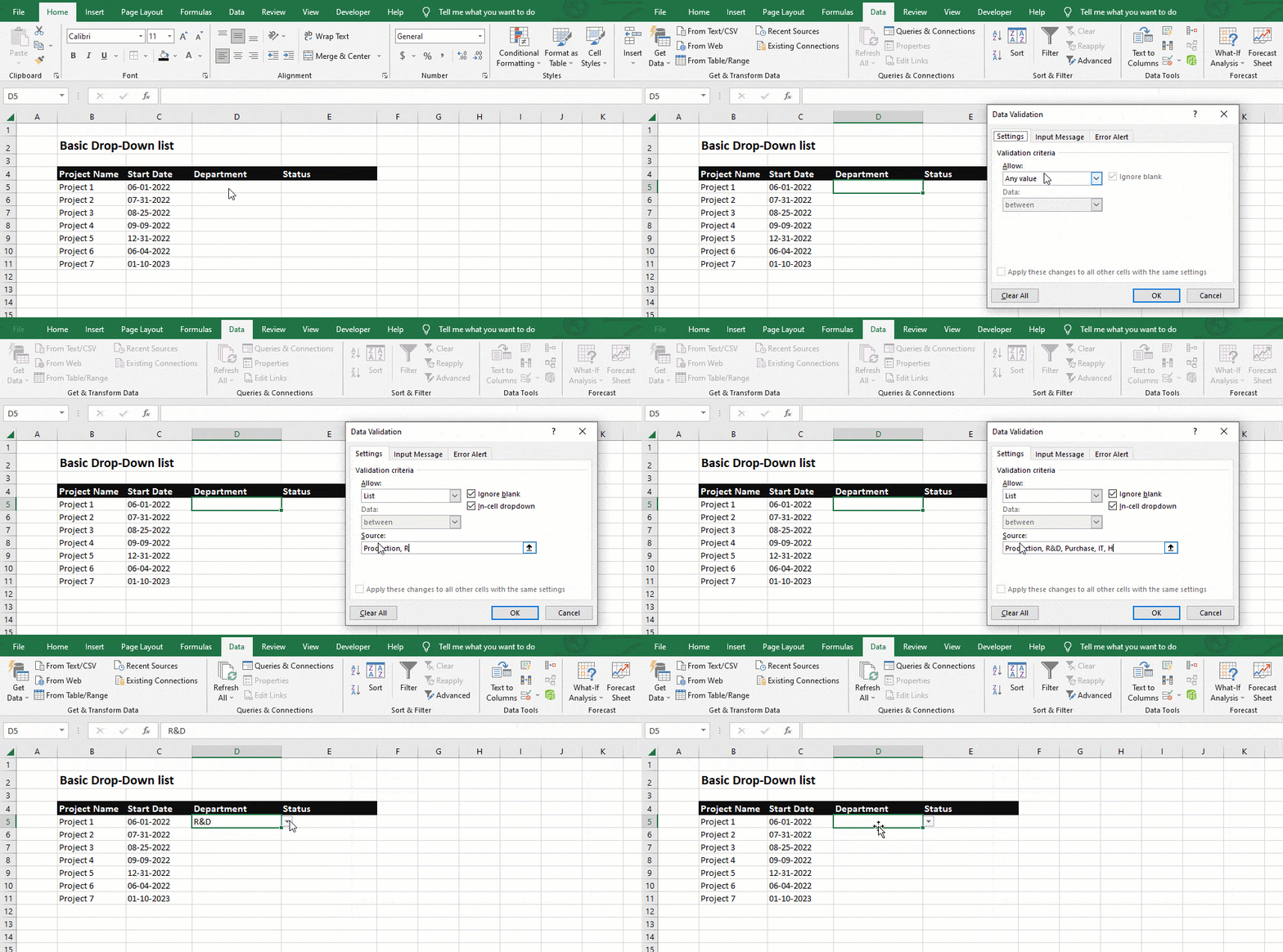
You can change that item at any time by selecting another item from the drop-down list or if you want to delete the cell content, just press the delete key on your keyboard.

How to make a drop-down list by selecting a range of cells

In that case, it can be a more easiest and most effective way to define the list on the listed columns.

Click the Source field or the up arrow icon, and simply reference the list item range using your mouse that contains the list of items you want to appear in the drop-down list.

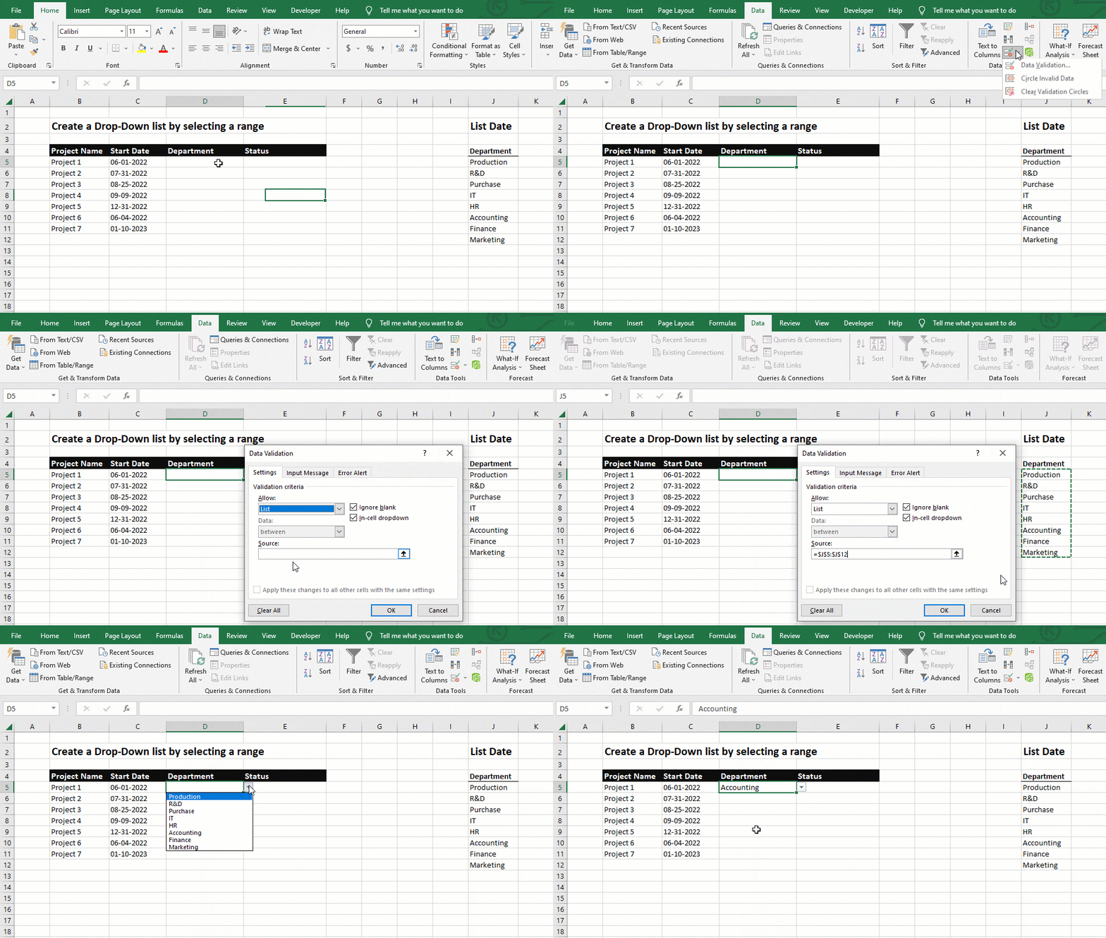
Once you click Ok, all the items in the reference range can now be selected in your drop-down list.

Rename/edit items from a Drop-Down list

Now if you want to rename an item from the list with this simple drop-down setup that was entered directly, Select the range and you would have to re-open the Data Validation window and change the items within this source field.

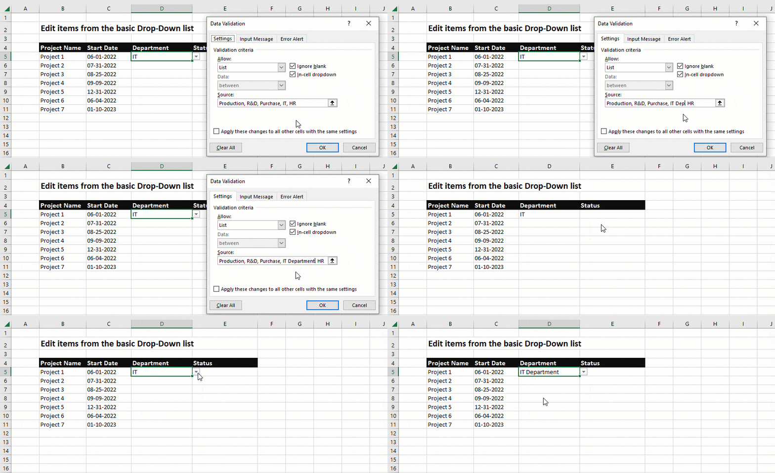
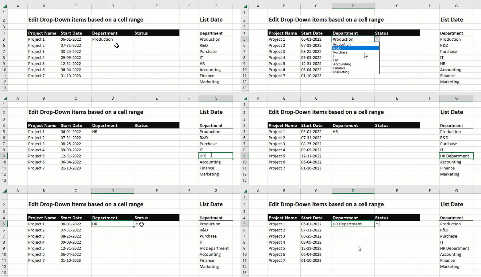
If you want to edit any of your items based on a cell range, it is much easier. As you can just go to the listed worksheet and change the item’s name in the cell directly. The changes will be automatically present in your drop-down list.

Show Input Message when the cell is selected

You can improve the user experience of a drop-down list by adding helpful input instructions.

Let’s say project a has multiple departments involved and the user filling out this sheet is not sure which of these involved departments should be selected.

To cover that scenario, you can add an input message that helps the user to make a selection.

For that, just open the Data Validation window with the cell selected, and in there go to the input message tab. Right at the top, you can control the visibility of the input message by checking the “Show input message when cell is selected” box, and below that’s the place to enter your message.

Let’s set up a helpful instruction for the department drop-down list.

For example,
Title: What to select here?
Input message: Please select the department that has the project lead.

Once we are ready, we click Ok.

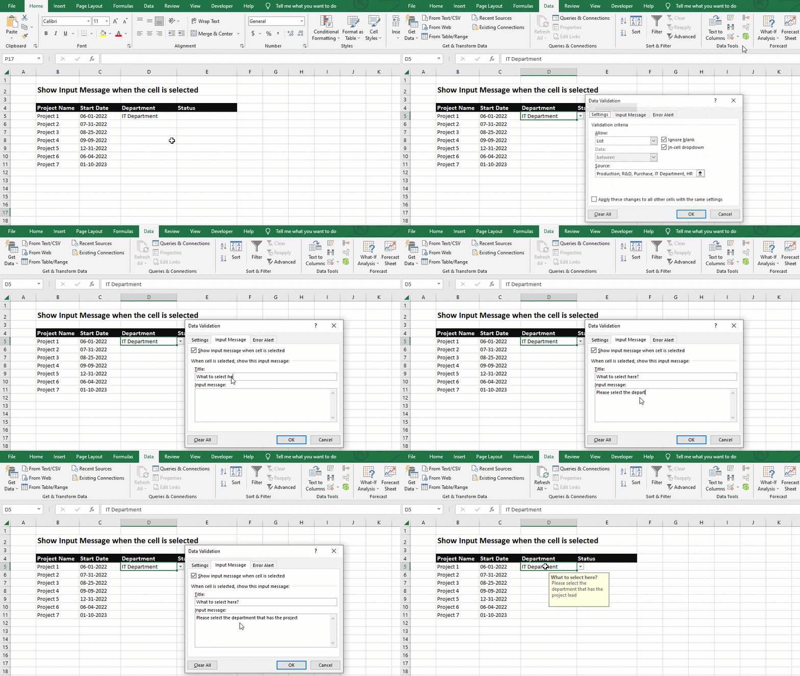
Now, whenever the cell with a drop-down list is selected the Input Message will be displayed to make it easier for the user, really amazing🤩

How to create a customized error alert in Excel

It doesn’t mean that is not possible to type values directly into the drop-down listed cell like other cells. Let’s try to type in a department that’s not on the list.

We get an instant error message. Because by default the data validation functionality of the drop-down list only allows values that have been defined items in the list.

If you want to allow other values into the cells to be entered. You can do that in the data validation options.

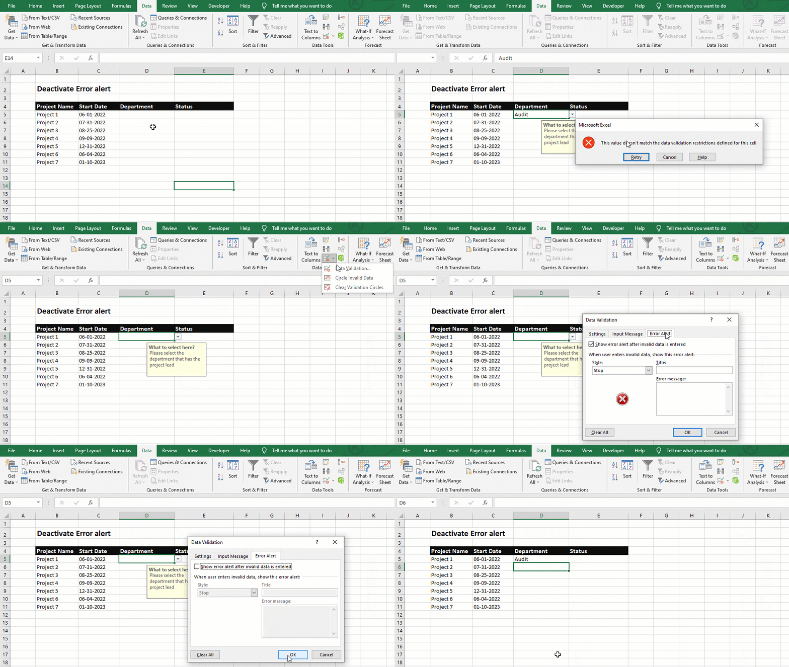
This time you need to go to the Third tab that says Error Alert. The “Show error alert after invalid data is entered” checkbox on top allows you to activate or deactivate the data validation completely.
Unchecking this box would mean we would enter any value without any validation or popup message.

But if you want to allow other values but still have some kind of control system.

You can change the style from Stop to Warning and click Ok and try again to enter any text.

This time a warning message popping up and now we can decide whether we want to continue or not.

The last style of data validation is Information. This will only bring up a notification that the value differs from the items on the list but no more questions are asked.

For most use cases, I recommend just leaving the default Stop style activated with customized this Error Message. So instead of having this generic error text. We can change that to something more useful.

For example,
Title: Unknown department.
Error message: Please select a department from the list.

After we are ready, then we click Ok.

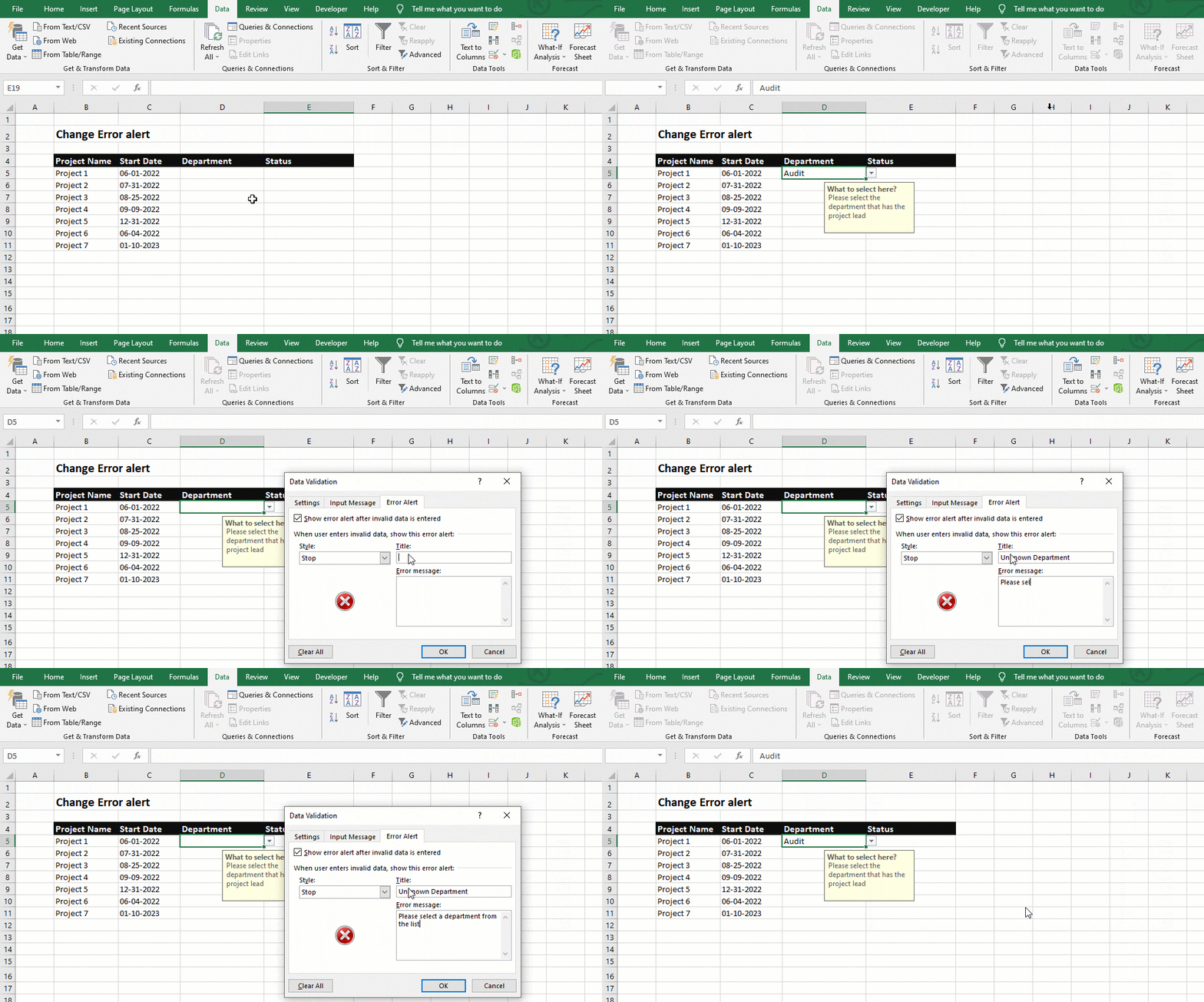
Now if we enter any text, we get this custom error message instead of that generic one, pretty cool😎

How to copy a drop-down list from one cell to another

We have set up these drop-down lists for the department’s first row. Now we want to copy the same drop-down lists in another cell as well. Let’s start: how??

There are basically two ways to quickly copy the drop-down functionality to these lower cells.

One way is to select the upper row and use the autocomplete function at the bottom right corner of the range to drag down.

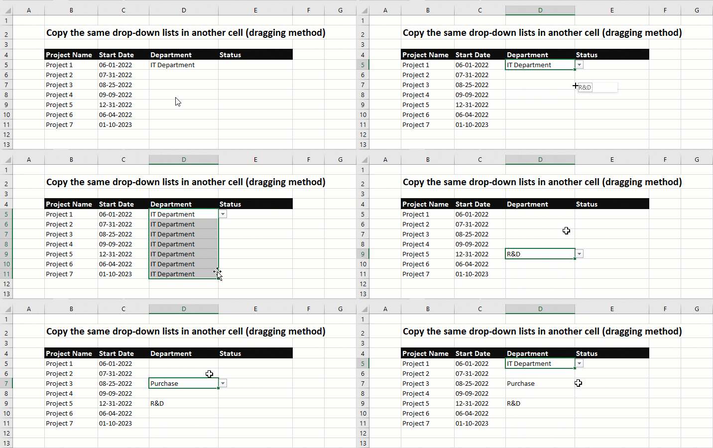
Note that:
That copies the drop-down lists but also the content that we have already selected. So with this method, we would need to clear everything if the cells are non-empty.

The second way is copy-paste method.

1. Select the first drop-down listed cell, and press Ctrl+C to copy.
2. Then select the rows below that you want to make the drop-down list.
3. Right-click and click on paste special. 
4. In the opening window, you have the option to select Validation and then click Ok.

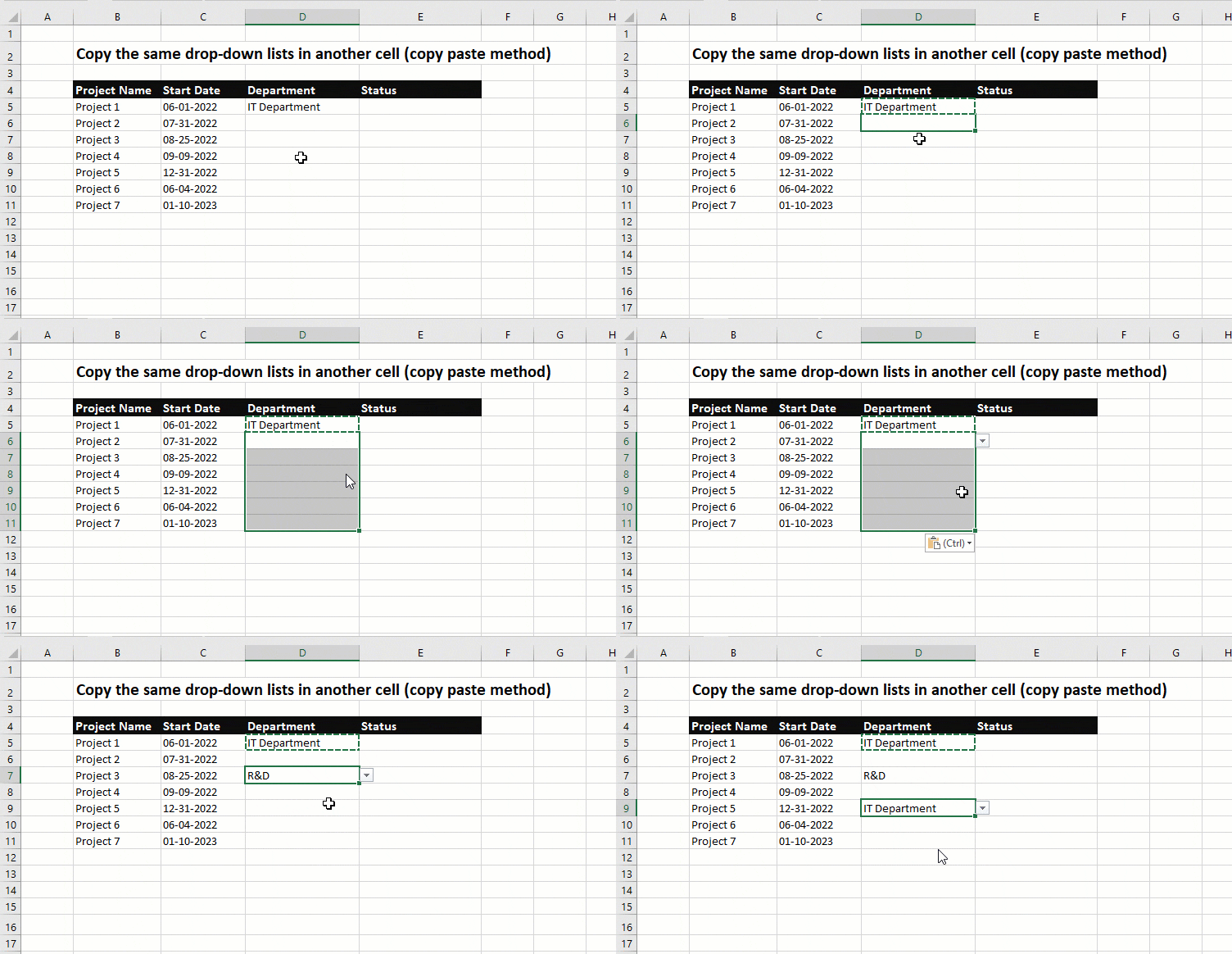
That way only the validation settings of the cells are copied down and everything works just fine.

Apply changes to other drop-down cells

Now that we have multiple cells with the same drop-down list.

We want to change the source reference for the drop-down list in one cell and these changes are applied to all other drop-down cells. Don’t worry, it’s actually pretty easy.

Just select one cell, open the Data validation window do whatever changes you want to do.

For example, let’s exclude these last two departments from the list, and if we now hit Ok, these changes would only apply to this one cell.

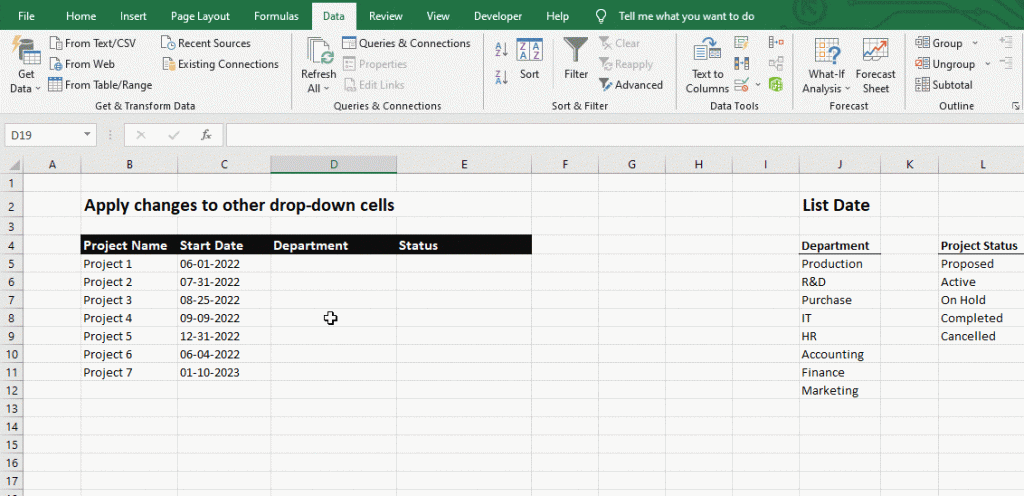
Instead, we check this option which says: Apply these changes to all other cells with the same settings and you see all these similar cells are automatically detected and if we click Ok, all department drop-down cells have an updated list of items.

At this point, we have covered all the fundamentals of drop-down lists in excel.